Introduction to yfinance: Fetching Historical Stock Data in Python

In today’s data-driven financial world, having access to reliable historical stock data is essential for in-depth market analysis and making informed investment decisions. Python, celebrated for its versatility and powerful data analysis libraries, has become a go-to language for financial data analysis. Among the various tools available, yfinance stands out as a simple yet powerful library that provides an easy-to-use interface for downloading historical market data from Yahoo Finance. This article offers a comprehensive introduction to yfinance, guides you through its setup, and demonstrates how to fetch, analyze, and visualize historical stock data.

What is yfinance?

yfinance is an open-source Python library designed to simplify the process of downloading financial data. Originally developed to address limitations in Yahoo Finance's official API, yfinance offers a reliable and efficient way to retrieve stock prices, company financials, and other market indicators. Whether you are a seasoned financial analyst or a programming newcomer, yfinance makes complex financial data easily accessible for further analysis using familiar Python tools.

Key features of yfinance include:

• Historical Data Retrieval: Obtain detailed historical stock data including Open, High, Low, Close, Volume, Dividends, and Stock Splits.
• Multiple Ticker Support: Fetch data for one or more stock symbols simultaneously.
• Company Insights: Retrieve additional financial metrics such as earnings, sustainability measures, and balance sheet information.
• Integration with Pandas: Data is returned as a pandas.DataFrame, allowing you to seamlessly integrate with the powerful data manipulation capabilities of Pandas.

Setting Up yfinance

Before you can start fetching financial data, you need to install the yfinance package. Installation is straightforward using pip:

pip install yfinance

Once installed, you can import yfinance in your Python script:

import yfinance as yf

This simple step prepares you to begin downloading and analyzing market data.

Fetching Historical Stock Data

One of the core functionalities of yfinance is its ability to download historical stock data. Let’s walk through a basic example of fetching historical data for Apple Inc. (ticker: AAPL).

Example: Fetching Apple Inc. Stock Data

# Import yfinance
import yfinance as yf

# Create a ticker object for Apple Inc.
apple = yf.Ticker('AAPL')

# Fetch historical stock data from January 1, 2020 to January 1, 2023
historical_data = apple.history(start='2020-01-01', end='2023-01-01')

# Display the retrieved data
print(historical_data)

In this example, a ticker object is created for Apple Inc. Using the history method, data from January 1, 2020, to January 1, 2023, is downloaded. The resulting DataFrame includes daily Open, High, Low, Close, Volume, and Dividend information, providing a detailed view of the stock’s historical performance.

Sample output:

                                 Open        High         Low       Close     Volume  Dividends  Stock Splits
Date                                                                                                         
2020-01-02 00:00:00-05:00   71.799873   72.856613   71.545387   72.796021  135480400        0.0           0.0
2020-01-03 00:00:00-05:00   72.020447   72.851776   71.862907   72.088310  146322800        0.0           0.0
2020-01-06 00:00:00-05:00   71.206092   72.701515   70.954024   72.662735  118387200        0.0           0.0
2020-01-07 00:00:00-05:00   72.672409   72.929322   72.100418   72.320976  108872000        0.0           0.0
2020-01-08 00:00:00-05:00   72.022865   73.787323   72.022865   73.484360  132079200        0.0           0.0
...                               ...         ...         ...         ...        ...        ...           ...
2022-12-23 00:00:00-05:00  129.557588  131.041978  128.290909  130.487808   63814900        0.0           0.0
2022-12-27 00:00:00-05:00  130.012807  130.042493  127.380484  128.676849   69007800        0.0           0.0
2022-12-28 00:00:00-05:00  128.320592  129.666440  124.560142  124.728371   85438400        0.0           0.0
2022-12-29 00:00:00-05:00  126.658071  129.122157  126.400782  128.261215   75703700        0.0           0.0
2022-12-30 00:00:00-05:00  127.073679  128.597646  126.103875  128.577850   77034200        0.0           0.0

[756 rows x 7 columns]

Analyzing and Manipulating the Data with Pandas

Because yfinance returns data in a pandas.DataFrame, you can leverage Pandas’ robust data manipulation tools for further analysis. For instance, calculating a moving average is a common task in financial analysis.

Example: Calculating a 20-Day Moving Average

# Calculate the 20-day moving average of Apple's closing price
moving_average = historical_data['Close'].rolling(window=20).mean()

# Add the moving average as a new column in the DataFrame
historical_data['20 Day MA'] = moving_average

# Display the updated DataFrame
print(historical_data.tail())

In this snippet, a 20-day moving average is computed for Apple’s closing prices using Pandas’ rolling method. This new column can help identify trends and smooth out short-term fluctuations, offering insights into the stock’s longer-term performance.

Visualizing Stock Data

Visual representation of data is key to understanding market trends. You can easily integrate yfinance with visualization libraries like Matplotlib or Seaborn.

Example: Plotting Closing Prices with Moving Average

Install matplotlib:

 pip install matplotlib

Full code:

import matplotlib.pyplot as plt

# Import yfinance
import yfinance as yf

# Create a ticker object for Apple Inc.
apple = yf.Ticker('AAPL')

# Fetch historical stock data from January 1, 2020 to January 1, 2023
historical_data = apple.history(start='2020-01-01', end='2023-01-01')

# Calculate the 20-day moving average of Apple's closing price
moving_average = historical_data['Close'].rolling(window=20).mean()

# Add the moving average as a new column in the DataFrame
historical_data['20 Day MA'] = moving_average


# Plot the closing prices and the 20-day moving average
plt.figure(figsize=(12, 6))
plt.plot(historical_data.index, historical_data['Close'], label='Close Price')
plt.plot(historical_data.index,
         historical_data['20 Day MA'], label='20 Day MA', linestyle='--')
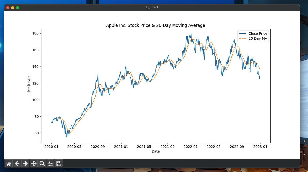
plt.title('Apple Inc. Stock Price & 20-Day Moving Average')
plt.xlabel('Date')
plt.ylabel('Price (USD)')
plt.legend()
plt.show()

This code creates a clear line chart comparing Apple’s closing prices with its 20-day moving average, providing a visual cue to help identify trends and potential buy or sell signals.

Screenshot:

Managing Multiple Tickers

yfinance also supports downloading data for multiple tickers in one go, which is particularly useful for portfolio analysis or comparative studies.

Example: Downloading Data for Multiple Stocks

# Download historical data for Apple, Microsoft, and Google
stocks = yf.download('AAPL MSFT GOOGL', start='2020-01-01', end='2023-01-01')

# Display the first few rows of the multi-index DataFrame
print(stocks.head())

In this example, the download method is used to fetch data for Apple (AAPL), Microsoft (MSFT), and Google (GOOGL) over the same historical period. The resulting DataFrame will have a multi-level column index, making it convenient to compare the performance of these stocks side by side.

Advanced Features and Financial Metrics

Beyond historical stock prices, yfinance can retrieve a wide range of financial metrics and company-specific data. This includes details like earnings calendars, balance sheets, and sustainability metrics.

Example: Retrieving Additional Company Information

# Fetch additional company information for Apple
apple_info = apple.info

# Fetch the earnings calendar for Apple
earnings_calendar = apple.calendar

# Display the company information and earnings calendar
print("Company Information:")
print(apple_info)
print("\nEarnings Calendar:")
print(earnings_calendar)

This section of the code demonstrates how to access comprehensive information about a company, such as market capitalization, sector details, and upcoming earnings dates. Such information is invaluable when performing due diligence or creating a detailed financial analysis report.

Error Handling and Best Practices

While yfinance is user-friendly, it’s important to incorporate error handling into your code to manage potential issues such as network errors, missing data, or changes in Yahoo Finance's data structure.

Example: Basic Error Handling

try:
    # Attempt to fetch historical data
    historical_data = apple.history(start='2020-01-01', end='2023-01-01')
except Exception as e:
    print("An error occurred while fetching data:", e)

Implementing error handling ensures that your application can gracefully manage unexpected issues and provide meaningful feedback to the user.

Integrating yfinance with Your Data Analysis Workflow

yfinance’s seamless integration with Pandas and visualization libraries means it can be a cornerstone in your data analysis workflow. Whether you are:

• Conducting Technical Analysis: Use historical data to calculate indicators such as moving averages, Bollinger Bands, and RSI.
• Performing Quantitative Research: Combine stock data with statistical libraries like NumPy and SciPy for complex analyses.
• Building Financial Models: Leverage the historical and real-time data capabilities of yfinance to create predictive models and backtesting systems.

By incorporating yfinance into your Python projects, you can develop robust financial tools tailored to your analytical needs.

Conclusion

yfinance is an indispensable tool for anyone interested in financial data analysis. Its ease of use, combined with the powerful data manipulation capabilities of Pandas, makes it a valuable resource for fetching historical stock data, analyzing market trends, and integrating financial metrics into your projects. Whether you are a financial professional, a data scientist, or a hobbyist looking to explore the stock market, yfinance provides the building blocks necessary for creating sophisticated and insightful analyses.

By following this guide, you now have a solid foundation to start exploring the capabilities of yfinance. From simple data downloads to advanced financial analytics and visualization, yfinance opens the door to a deeper understanding of the financial markets—all through the power of Python.

Happy coding and insightful investing!